Optimization Resources
A collection of software and resources for nonlinear optimization.
Maintained by Coralia Cartis (University of Oxford), Jaroslav Fowkes (STFC Rutherford Appleton Laboratory) and Lindon Roberts (Australian National University).
Optimization Software and Online Resources
There are many software packages for solving optimization problems. Here we provide a list of some available solvers that we have developed and a number of other packages that are available for solving a broad variety of problems in several programming languages. On this page we focus on nonlinear optimization (not other important categories such as linear programming or integer programming problems).Nonlinear Optimization Problems
These problems take the form $$ \min_{x\in\mathbb{R}^n} f(x), $$ where $f$ is an 'objective' function (implemented as a piece of code) which takes the length-$n$ array $x$ of continuous variables and computes some quantity of interest depending on $x$. If the problem is to maximize $f$, then you can instead minimize $(-1)\times f(x)$ to put it in the form required by most solvers.Constraints
It is often the case that the variables $x$ can only take some values, and we call such problems constrained: $$ \min_{x\in\Omega} f(x), $$ where $\Omega$ is some region of $n$-dimensional space defining the valid choices of $x$. This 'feasible region' is usually represented by a collection of constraint functions of the form $c(x)\geq 0$ or $c(x)=0$. Some simple constraints are sometimes considered explicitly, such as box constraints $a_i \leq x_i \leq b_i$ (i.e. the $i$-th entry of $x$ must be between $a_i$ and $b_i$). In general it is better to represent constraints in the simplest possible way (e.g. don't use $e^x \leq 1$ when you could use $x\leq 0$ instead).Data Fitting/Inverse Problems
One very common special type of optimization problem is nonlinear least-squares problems, which are very common in data fitting and inverse problems. In this case, the objective function has the special form $$ f(x) = \sum_{i=1}^{m} r_i(x)^2, $$ where each function $r_i(x)$ usually represents a fitting error corresponding to the $i$-th data point (out of $m$ total data points).Problem Information to Supply
What information you have access to can determine what type of solver you should use. In general, most solvers will require you to provide a piece of code which computes $f(x)$ for any $x$ (and $c(x)$ for any constraints). Usually you will also need to be able to compute the gradient of the objective (and all constraints), that is provide code which returns the $n$-dimensional vector $\nabla f(x)$ for any $x$ (where the $i$-th entry of $\nabla f(x)$ is the derivative of $f$ with respect to the $i$-th entry of $x$). You can implement a gradient calculation by explicitly calculating the derivatives (if you know the explicit mathematical form of $f$), or use finite differencing techniques or algorithmic differentiation software packages.
For nonlinear least-squares problems and problems with multiple constraints, often you will need to write code to return a vector of results (e.g. given $x$, return the length-$m$ vector $r(x)=[r_1(x) \: \cdots \: r_m(x)]$ for nonlinear least-squares problems). In this case, instead of the gradient $\nabla f(x)$ you will need to provide the Jacobian matrix of first derivatives. For instance, if you have a function $r(x)=[r_1(x) \: \cdots \: r_m(x)]$ where $x$ has $n$ entries, the Jacobian matrix has $m$ rows and $n$ columns and the $i$-th row is $\nabla r_i(x)$.
Some solvers also allow you to provide code to calculate the second derivatives of $f$ (the Hessian of $f$), but this is usually not necessary. In general the more information you can provide, the better the optimization solver will perform, so it is sometimes worth the effort of writing Hessian code.
If you are writing code which returns very large matrices (e.g. Jacobians or Hessians), it is often useful to think about the sparsity of these matrices: which entries are always zero for every $x$? Many solvers allow you to provide Jacobians or Hessians as sparse matrices, which can give substantial savings on memory and computation time.
If your calculation of $f$ has some randomness (e.g. it requires a Monte Carlo simulation) or is very computationally expensive, then evaluating $\nabla f(x)$ may be very expensive or inaccurate. In this case, you may want to consider derivative-free solvers, which only require code to evaluate $f$.
Our Software
- DFO-LS (open source, Python) - a derivative-free nonlinear least-squares solver (i.e. no first derivatives of the objective are required or estimated), with optional bound constraints. This solver is suitable when objective evaluations are expensive and/or have stochastic noise, and has many input parameters which allow it adapt to these problem types. It is based on our previous solver DFO-GN.
- oBB (open source, Python) - a parallelized solver for global optimization problems with general constraints. It requires first derivatives of the objective and bounds on its second derivatives. It is part of the COIN-OR collection (see below).
- P-IPM-LP (open source, MATLAB) - a perturbed Interior Point Method for linear programming problems (i.e. minimize a linear function subject to linear constraints).
- Py-BOBYQA (open source, Python) - a derivative-free general objective solver, with optional bound constraints. The algorithm is based on Mike Powell's original BOBYQA (Fortran), but includes a number of the features from DFO-LS, which improve its performance for noisy problems.
- trustregion (open source, Python) - a wrapper to Fortran routines for solving the trust-region subproblem. This subproblem is an important component of some optimization solvers.
Other Software Packages
These are some software packages which we have had some involvement with, directly or indirectly.
- COIN-OR (open source, many languages) - an organization which maintains a collection of many open-source optimization packages for a wide variety of problems. A list of packages by problem type is here and the source code is on Github.
- FitBenchmarking (open source, Python) - a tool for comparing different optimization software for data fitting problems. The documentation is here and the source code is on Github.
- GALAHAD (open source, Fortran with C, MATLAB, Python and Julia interfaces) - a collection of routines for constrained and unconstrainted nonlinear optimization, including useful subroutines such as trust-region and cubic regularization subproblem solvers. The source code is on Github.
- NAG Library (proprietary, many languages) - a large collection of mathematical software, inluding optimization routines for many problem types (nonlinear, LPs, QPs, global, mixed integer, etc.). Note: some of our research has been partially supported by NAG.
Other Resources and Software
Software packages:
- Ipopt (open source, C++ with interfaces to many languages including Python, MATLAB, C and Julia) - a package for solving inequality-constrained nonlinear optimization problems.
- Julia Smooth Optimizers and JuliaOpt (open source, Julia) - a collection of packages for optimization, including solvers, profiling tools (such as creating performance profiles) and a CUTEst interface.
- KNitro (proprietary, free trial available, MATLAB) - a high quality solver for general constrained and unconstrained nonlinear optimization problems.
- NLOpt (open source, many languages including Python, MATLAB, Fortran and C) - a library which wraps many different nonlinear optimization solvers in a unified interface. Solvers include SQP, augmented Lagrangian and L-BFGS (local), DIRECT (global) and BOBYQA (local, derivative-free).
- RALFit (open source, Fortran with interfaces to C and Python) - a package for solving nonlinear least-squares problems (such as some data fitting and inverse problems).
Other resources:
- arXiv:math.OC - a repository of optimization-related preprints.
- Decision Tree for Optimization Software - an extensive database of software for many different types of optimization problem, carefully sorted by problem type.
- Global Optimization test problems - a collection of resources maintained by Arnold Neumaier (University of Vienna).
- NEOS server - an online server where you can submit jobs to be solved by specific solvers.
- NEOS guide - a reference page with explanations of the different types of optimization problems and summaries of many key algorithms (sorted by problem type). It also has its own page of optimization resources, such as key journals and conferences.
- Optimization Online - a repository of optimization-related preprints.
Optimization Test Problems
This section gives details of how to install the extensive CUTEst library of optimization test problems (paper) - earlier versions were called CUTE (1995) and CUTEr (2003) - as well as providing some standard collections of optimization test problems. CUTEst is a Fortran library, but we give instructions for installing wrappers for Matlab and Python. The other problem sets are implemented in Python.
CUTEst for Linux
To use CUTEst on Linux you will need to install four packages: archdefs, SIFDecode, CUTEst and MASTSIF. To keep things simple, install all four packages in the same directory:
					mkdir cutest
					cd cutest
					git clone https://github.com/ralna/ARCHDefs ./archdefs
					git clone https://github.com/ralna/SIFDecode ./sifdecode
					git clone https://github.com/ralna/CUTEst ./cutest
					git clone https://bitbucket.org/optrove/sif ./mastsif
mastsif contains all the test problem definitions and is therefore quite large.
If you're short on space you may want to copy only the *.SIF files for the problems you wish to test on.
Next set the following environment variables in your ~/.bashrc to point to the installation directories used above:
					# CUTEst
					export ARCHDEFS=/path/to/cutest/archdefs/
					export SIFDECODE=/path/to/cutest/sifdecode/
					export MASTSIF=/path/to/cutest/mastsif/
					export CUTEST=/path/to/cutest/cutest/
					export MYARCH="pc64.lnx.gfo"
					export MYMATLAB=/path/to/matlab/ # if using Matlab interface
				        source ~/.bashrc # load above environment variables
				        cd ./cutest
				        $ARCHDEFS/install_optrove
					Do you wish to install CUTEst (Y/n)? y
					Do you require the CUTEst-Matlab interface (y/N)? y # if using Matlab interface (see below)
					Select platform: # PC with generic 64-bit processor
					Select operating system: # Linux
					Select Matlab version: # R2016b or later
					Would you like to compile SIFDecode ... (Y/n)? y
					Would you like to compile CUTEst ... (Y/n)? y
					CUTEst may be compiled in (S)ingle or (D)ouble precision or (B)oth.
					Which precision do you require for the installed subset (D/s/b) ? D
Installing the Python Interface
To obtain a Python interface to CUTEst, please install PyCUTEst: https://github.com/jfowkes/pycutestCUTEst for Mac
To use CUTEst on Mac you will first need to install the Homebrew package manager:
/bin/bash -c "$(curl -fsSL https://raw.githubusercontent.com/Homebrew/install/HEAD/install.sh)"
					brew tap optimizers/cutest
					brew install cutest --without-single --with-matlab # if using Matlab interface
					brew install mastsif  # if you want all the test problems
					for f in "archdefs" "mastsif" "sifdecode" "cutest"; do \
					echo ". $(brew --prefix $f)/$f.zshrc" >> ~/.zshrc; \
					done
~/.zshrc, e.g.,
export MYMATLAB=/Applications/MATLAB_R2023b.app
Installing the Python Interface
To obtain a Python interface to CUTEst, please install PyCUTEst: https://github.com/jfowkes/pycutestInstalling the Matlab Interface on Apple Silicon Macs
This is rather involved unfortunately. First ensure that you have installed the Apple Silicon version of Matlab (and not the Intel Mac version). Then download the shell script below and place it somewhere on yourPATH. I like to create ~/bin and add it to my PATH. Make the script executable:
					mkdir ~/bin  # if not already done
					cp Downloads/cutest2matlab_macos.sh ~/bin/
					chmod +x ~/bin/cutest2matlab_macos.sh
					export PATH=~/bin:$PATH  # if not already done; add this to your ~/.zshrc
cutest2matlab_macos.sh:
					mkdir rosenbrock
					cd rosenbrock
					cutest2matlab_macos.sh ROSENBR
					libROSENBR.dylib
					mcutest.mexmaca64
					addpath('/opt/homebrew/opt/cutest/libexec/src/matlab')
					cd /the/directory/where/you/ran/cutest2matlab_macos.sh
					prob = cutest_setup()
f = cutest_obj(prob.x)
Installing the Matlab Interface on Legacy Intel Macs
This is even more involved unfortunately. First download the following xml file and place it in~/Library/Application\ Support/Mathworks/MATLAB/R2018a/ (substitute your Matlab version).
Then download the shell script below
and place it somewhere on your PATH. I like to create ~/bin and add it to my PATH. Make the script executable:
					mkdir ~/bin  # if not already done
					cp Downloads/cutest2matlab_osx.sh ~/bin/
					chmod +x ~/bin/cutest2matlab_osx.sh
					export PATH=~/bin:$PATH  # if not already done; add this to your ~/.zshrc
cutest2matlab_osx.sh:
					mkdir rosenbrock
					cd rosenbrock
					cutest2matlab_osx.sh ROSENBR
					libROSENBR.dylib
					mcutest.mexmaci64
					addpath('/usr/local/opt/cutest/libexec/src/matlab')
					cd /the/directory/where/you/ran/cutest2matlab_osx.sh
					prob = cutest_setup()
f = cutest_obj(prob.x)
CUTEst for Windows
The easiest way to set up CUTEst and PyCUTEst on Windows is to install the Windows Subsystem for Linux (on Windows 10 or 11). This gives you access to a Linux filesystem and a bash terminal, from which you can install regular programs such as Python and gfortran (using apt-get), and install CUTEst/PyCUTEst using the Linux instructions above.Running Linux GUIs
It is possible to run Linux GUI programs too, but this is not enabled by default. For this, you need to:
- Install an X-server program on Windows (e.g. VcXsrv or see here for others).
- Ensure the X-server is running (you may want to enable it to start automatically on Windows startup).
- Modify your
.bashrcfile in your Linux file system to include the linesexport DISPLAY=localhost:0.0 export LIBGL_ALWAYS_INDIRECT=1 - Install the WSL utilities program in Linux (e.g.
apt-get install wslu). - Use the installed Linux program
wsluscto create a shortcut in Windows to start your desired GUI application (runman wsluscin bash for instructions). Alternatively, you can do this manually by creating a.batWindows script file which contains (if you have Ubuntu 18.04)
making sure to include yourC:\Windows\System32\wscript.exe C:\\Users\\username\wslu\runHidden.vbs C:\\Users\\username\\AppData\\Local\\Microsoft\\WindowsApps\\CanonicalGroupLimited.Ubuntu18.04onWindows_79rhkp1fndgsc\\ubuntu1804.exe run "cd ~; . /usr/share/wslu/wsl-integration.sh; /path/to/gui/executable; "C:\\Users\\usernamedirectory and edit the/path/to/gui/executable. You should double-check the path to your Linux executable to make sure this runs. Double-click on the.batfile to execute it.
Python interface for CUTEst
To obtain a Python interface to CUTEst, please install PyCUTEst: https://github.com/jfowkes/pycutest
Moré-Garbow-Hillstrom Test Collection
The Moré-Garbow-Hillstrom (MGH) test collection has a number of common unconstrained nonlinear least-squares test problems. To install the MGH test set for Python, please download the following file: and place it in the same directory as your Python code requiring the test problems.Using the test set
To create an instance of the extended Rosenbrock function and evaluate the residual and Jacobian at the initial point:
					from MGH import ExtendedRosenbrock
					rb = ExtendedRosenbrock(n=4, m=4)
					x0 = rb.initial # initial point
					rb.r(x0) # residual vector at x0
					rb.jacobian(x0) # Jacobian at x0
Moré & Wild Test Collection
The Moré & Wild (MW) test collection is a collection of common unconstrained nonlinear least-squares problems, designed for testing derivative-free optimization solvers. To install the MW test set for Python, please download the following two files: and place them in the same directory as your Python code requiring the test problems. The code can provide either the vector of residuals or the full least-squares objective. More details of the problems, including an estimate of f_min, are given in the associated more_wild_info.csv file.Using the test set
Choose a problem number from 1 to 53 and then either get the scalar objective function:
					from more_wild import *
					f, x0, n, m = get_problem_as_scalar_objective(probnum)
					from more_wild import *
					r, x0, n, m = get_problem_as_residual_vector(probnum)
- f is the scalar objective $f(\mathbf{x})=r_1(\mathbf{x})^2 + \cdots + r_m(\mathbf{x})^2$
- r is the vector of residuals $r(\mathbf{x}) = [r_1(\mathbf{x}) \: \cdots \: r_m(\mathbf{x})]$
- x0 is the initial starting point for the solver
- n is the dimension of the problem
- m is the number of residuals in the objective
Creating stochastic problems
The code also allows you to create stochastic problems by adding artificial random noise to each evaluation of $f(\mathbf{x})$ or $r(\mathbf{x})$. You do this by calling one of:
					from more_wild import *
					r, x0, n, m = get_problem_as_residual_vector(probnum, noise_type='multiplicative_gaussian', noise_level=1e-2)
					f, x0, n, m = get_problem_as_scalar_objective(probnum, noise_type='multiplicative_gaussian', noise_level=1e-2)
noise_type are:
smooth(default): no noise addedmultiplicative_deterministic: each $r_i(\mathbf{x})$ is replaced by $\sqrt{1+\sigma \phi(\mathbf{x})} r_i(\mathbf{x})$, where $\sigma$ is equal tonoise_leveland $\phi(\mathbf{x})$ is a deterministic high frequency function taking values in $[-1,1]$ (see equation (4.2) of the Moré & Wild paper). The resulting function is still deterministic, but it is no longer smooth.multiplicative_uniform: each $r_i(\mathbf{x})$ is replaced by $(1+\sigma) r_i(\mathbf{x})$, where $\sigma$ is uniformly distributed between-noise_levelandnoise_level(sampled independently for each $r_i(\mathbf{x})$).multiplicative_gaussian: each $r_i(\mathbf{x})$ is replaced by $(1+\sigma) r_i(\mathbf{x})$, where $\sigma$ is normally distributed with mean 0 and standard deviationnoise_level(sampled independently for each $r_i(\mathbf{x})$).additive_gaussian: each $r_i(\mathbf{x})$ is replaced by $r_i(\mathbf{x}) + \sigma$, where $\sigma$ is normally distributed with mean 0 and standard deviationnoise_level(sampled independently for each $r_i(\mathbf{x})$).additive_chi_square: each $r_i(\mathbf{x})$ is replaced by $\sqrt{r_i(\mathbf{x})^2 + \sigma^2}$, where $\sigma$ is normally distributed with mean 0 and standard deviationnoise_level(sampled independently for each $r_i(\mathbf{x})$).
Methodology for Comparing Solvers
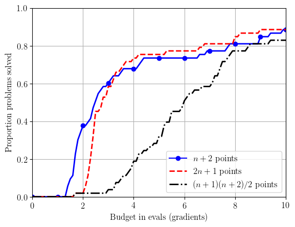
This section contains details about data and performance profiles, two common approaches for comparing different optimization solvers' performance on a collection of test problems. We describe the methodology, and provide Python software for generating these profiles.Data & Performance Profiles
To compare solvers, we use data and performance profiles as defined by Moré & Wild (2009). First, for each solver $\mathcal{S}$, each problem $p$ and for an accuracy level $\tau\in(0,1)$, we determine the number of function evaluations $N_p(\mathcal{S};\tau)$ required for a problem to be `solved': $$ N_p(\mathcal{S}; \tau) := \text{# objective evals required to get $f(\mathbf{x}_k) \leq f^* + \tau(f(\mathbf{x}_0) - f^*)$,} $$ where $f^*$ is an estimate of the true minimum $f(\mathbf{x}^*)$. (Note: sometimes $f^*$ is taken to be the best value achieved by any solver.) We define $N_p(\mathcal{S}; \tau)=\infty$ if this was not achieved in the maximum computational budget allowed. This measure is suitable for derivative-free solvers (where no gradients are available), but alternative measures of success can be used if gradients are available (see next section).
We can then compare solvers by looking at the proportion of test problems solved for a given computational budget. For data profiles, we normalise the computational effort by problem dimension, and plot (for solver $\mathcal{S}$, accuracy level $\tau\in(0,1)$ and problem suite $\mathcal{P}$) $$ d_{\mathcal{S}, \tau}(\alpha) := \frac{|\{p\in\mathcal{P} : N_p(\mathcal{S};\tau) \leq \alpha(n_p+1)\}|}{|\mathcal{P}|}, \qquad \text{for $\alpha\in[0,N_g]$,} $$ where $N_g$ is the maximum computational budget, measured in simplex gradients (i.e. $N_g(n_p+1)$ objective evaluations are allowed for problem $p$).
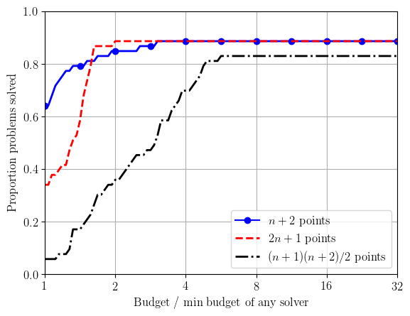
For performance profiles (originally proposed by Dollan & Moré (2002)), we normalise the computational effort by the minimum effort needed by any solver (i.e. by problem difficulty). That is, we plot $$ \pi_{\mathcal{S},\tau}(\alpha) := \frac{|\{p\in\mathcal{P} : N_p(\mathcal{S};\tau) \leq \alpha N_p^*(\tau)\}|}{|\mathcal{P}|}, \qquad \text{for $\alpha\geq 1$,} $$ where $N_p^*(\tau) := \min_{\mathcal{S}} N_p(\mathcal{S};\tau)$ is the minimum budget required by any solver.
When multiple test runs are used, we take average data and performance profiles over multiple runs of each solver; that is, for each $\alpha$ we take an average of $d_{\mathcal{S},\tau}(\alpha)$ and $\pi_{\mathcal{S},\tau}(\alpha)$. When plotting performance profiles, we took $N_p^*(\tau)$ to be the minimum budget required by any solver in any run.
Measuring Performance for Gradient-Based Solvers
The above was designed comparing derivative-free solvers, where gradients are not available. If, however, derivative information is available, it may be better to replace the definition above with $$ N_p(\mathcal{S}; \tau) := \text{# objective evals required to get $\|\nabla f(\mathbf{x}_k)\| \leq \tau \|\nabla f(\mathbf{x}_0)\|$.} $$ The above script can handle this definition by a modification of the input files:
- In the problem information, replace columns 'f0' and 'fmin (approx)' with $\|\nabla f(\mathbf{x}_0)\|$ and 0 respectively;
- The last column of the raw solver results should be $\|\nabla f(\mathbf{x}_k)\|$ instead of $f(\mathbf{x}_k)$ for each evaluation.
Plotting Code
We provide methods for generating data and performance profiles, plus a script with example usage: These methods assume you have results for a single solver for a collection of test problems in a text file, with format
Problem number, evaluation number, objective value
				1,1,71.999999999999986
				1,2,72.410000006258514
				...
				53,89,1965397.5762139191
				53,90,1953998.3397798422
Processing Raw Results
A raw file in the format described above can be converted to the correct format using the following:
					from plotting import *
					problem_info_file = '../mw/more_wild_info.csv'  # problem suite information
					infile = 'raw_bobyqa_budget10_np2.csv'
					outfile = 'clean_bobyqa_budget10_np2.csv'
					solved_times = get_solved_times_for_file(problem_info_file, infile)
					solved_times.to_csv(outfile)
				Setting,n,fmin,nf,tau1,tau2,tau3,tau4,tau5,tau6,tau7,tau8,tau9,tau10
				1,9,36.0000000021001,100,18,29,41,49,54,64,71,85,93,98
				...
				53,8,1953998.3397798422,90,12,12,21,23,-1,-1,-1,-1,-1,-1
Generating Plots
To generate data and performance profiles, we first build a list of tuples containing plotting information. The first entry is the stem of the processed results file - if we provide stem, all files of the form stem*.csv are assumed to contain runs for that solver, and we use an average data/performance profile over all these runs. This is needed if the algorithm and/or objective evaluation has noise. We also need plot formatting information: legend label, line style, color and (optional) marker and marker size. These can be taken from the standard matplotlib options.
				    # each entry is tuple = (filename_stem, label, colour, linestyle, [marker], [markersize])
				    solver_info = []
				    solver_info.append(('clean_bobyqa_budget10_np2', r'$n+2$ points', 'b', '-', '.', 12))
				    solver_info.append(('clean_bobyqa_budget10_2np1', r'$2n+1$ points', 'r', '--'))
				    solver_info.append(('clean_bobyqa_budget10_nsq', r'$(n+1)(n+2)/2$ points', 'k', '-.'))
				    from plotting import *
				    tau_levels = [1, 3]
				    budget = 10
				    outfile_stem = 'demo'
				    # solver_info defined as above
				    create_plots(outfile_stem, solver_info, tau_levels, budget)
- max_ratio - A float for the largest x-axis value in performance profiles (default is 32.0);
- data_profiles - A boolean flag for whether to generate data profiles (default is True);
- perf_profiles - A boolean flag for whether to generate performance profiles (default is True);
- save_to_file - A boolean flag for whether to save plots to file; if False, plots are displayed on screen (default is True);
- fmt - A string for image output type, which needs to be accepted by matplotlib's savefig command (default is "eps");
- dp_with_logscale - A boolean flag for whether the x-axis for data profiles should be in a log scale (default is False).
- expected_nprobs - An integer with the number of problems in the test set (if provided, check all input files to ensure they have exactly this many problems)