The Perseus Software Project for Rapid Computation of Persistent Homology
Download or Compile
Click on the icon for your operating system in order to download the suitable executable file. The current version is 4.0 Beta.
| Microsoft Windows XP and above | 64 Bit | |
| Linux (Ubuntu, Mint, Debian, SuSE,...) | 64 Bit | |
| Mac OS Tiger and up | 64 Bit |
Once you have the file corresponding to your operating system, see "Basic Information and Usage" below. If you'd prefer to compile the software from source yourself instead, keep reading.
The source code is also available as a zipped file here. Download this to a directory where you have read/write permissions. You can now Use any C++ compiler to compile the main file Pers.cpp. The choice of compiler depends mainly on your operating system. Microsoft Windows users have various compiler options such as the open-source mingw, or the complete integrated development environment provided by the somewhat pricey Microsoft Visual Studio. Mac users will probably require a hefty Xcode download and installation on their systems.
If using the gcc compiler from the command line, just go to the directory with the extracted source files and type:
g++ Pers.cpp -O3 -fpermissive -o perseus
Of course, you can replace "perseus" in the command above with any executable name of your choice.
Warning for New Users: The current version may not be compatible with the Clang compiler (default on new Macs). If things are not working out on your machine, please consider either downloading a precompiled file or installing a gcc compiler!
To report a bug or to suggest a new feature, please send email by clicking here. It would really help speed things up if your subject line contained the word "Perseus" in it somewhere!
Basic Information and Usage
Perseus computes the persistent homology of many different types of filtered cell complexes after first performing certain homology-preserving Morse theoretic reductions. In all cases, the user should prepare the input filtration as a correctly-formatted text file (see instructions for formatting below) and then read the output persistent homology intervals, again presented as text files.
Since Perseus is based on discrete Morse theory, it does not rely on the idiosyncracies of a particular type of complex structure or dimension for its efficiency. That being said, certain types of complexes are much more common than others in the realm of data analysis. For dealing with movies and images, it is best to work with cubical data structures. On the other hand, if the data source is a manifold triangulation, then the appropriate representation consists of top-cell information on a simplicial complex. Point cloud data is usually handled effectively with Vietoris-Rips complexes built around those points.
To actually compute persistent homology of your input filtered complex, you will need to enter the following command line arguments (without parentheses) in the given order, either directly into a terminal or using your integrated development environment.
- (path to perseus executable) (complex type) (input filename) (output file string)
The (output file string) is completely optional, it simply provides a prefix for the output files so that they will be easy to locate and identify. So for instance if you are working on project DeathStar, then making the output string DeathStar produces output files which have a prefix DeathStar followed by other stuff. To parse the generated output files, see the box titled "Understanding and Visualizing the Output" below. For more details on acceptable (complex type)s and how to format the respective (input file)s, click on the appropriate input format box below for information about cubical, simplicial and other types of input complexes as well as simple examples for each complex type. Here is a little cheat-sheet with the most common complex types:
cubtop: for a dense cubical grid from top-level cube information.
scubtop: for a sparse cubical grid from top-level cube information.
simtop: for a simplicial complex from uniform top-level triangulation data.
nmfsimtop: for a general simplicial complex from non-uniform top-level simplex information.
rips: for a Vietoris-Rips complex from non-uniform birth point information.
brips: for a Vietoris-Rips complex from uniform birth point information.
distmat: for a Vietoris-Rips complex from a distance matrix.
As you can see, Perseus is equipped to handle a diverse variety of input complexes, and it is not too difficult to add front-ends for reading in new complex types that are not already present in one of the boxes below. There is also no restriction on dimension except system memory: simplices of dimension 70 have a lot of faces and sub-faces! The boxes below explain how to format simple text files to create the desired input complexes for Perseus. It is important to follow the file format strictly, so please check the provided example files in case of confusion.
Warning: While preparing your dataset for Perseus, you will most likely have occasion to enter "birth times" for various cells. In order to ensure that the software processes your complexes correctly, please avoid using 0 as a birth time.. Also do not use floating-point numbers or negative numbers for birth times (except -1 which has a specific purpose). Instead, just use 1, 2, 3,... and so on.
Persistent Homology of Cubical Toplexes
A toplex is a cell complex which can be constructed from a list of top dimensional cells. So, a cubical toplex of dimension d is just a list of d-dimensional cubes. The faces and subfaces of these cubes are constructed automatically from the top-cube information provided by input files. A simple way to represent a full-dimensional cube is to provide the coordinate of its lexicographically minimal vertex, which we will call its anchor. So, a 3D cube anchored at the point (a,b,c) with integer coordinates must be the cube with vertices of the form (a+i,b+j,c+k) where i, j and k are only allowed to take the values 0 and 1.
Perseus is presently able to compute the persistent homology of the following types of cubical data:
Dense Cubical Grids
A dense cubical grid of dimension d consists of integer-vertex cubes in d-dimensional Euclidean space. Each cube gets a birth-time, but if you are interested in computing the standard homology rather than the persistence then you can set all the birth times of cubes which appear to 1. By convention, a birth time of -1 is reserved for cubes that are missing from the grid.
The file format is straightforward. The first line contains the dimension of the cubical grid, let's say d. The next d lines of the file indicate the grid size along that dimension. Of course, these must be non-negative numbers. So to enter information about a four dimensional grid of 100 by 30 by 50 by 12 cubes, the first five lines of your file must be 4, 100, 30, 50 and 12 in that order. The lines after that contain the integer birth times of all the cubes in lexicographical order of anchor points, with preference given to the dimensions in their chosen order.

Here is an example text file containing a 2 dimensional 3 by 4 grid where the birth time of each 2D cube is the sum of the anchor coordinates, except in the case of the cube anchored at (1,1) which never appears in the complex at all and therefore gets a birth time of -1. Note that all indices start with 0 instead of 1. Here is an explanation of the numbers in this file:
2 : this is the dimension of the cubical grid
3 : this is the number of cubes along the first dimension
4 : this is the number of cubes along the second dimension
1 : this is the birth time of the 2D cube anchored at (0,0)
2 : this is the birth time of the 2D cube anchored at (1,0)
1 : this is the birth time of the 2D cube anchored at (2,0)
2 : this is the birth time of the 2D cube anchored at (0,1)
-1 : this indicates that there is no cube anchored at at (1,1)
2 : this is the birth time of the 2D cube anchored at (2,1)
1 : this is the birth time of the 2D cube anchored at (0,2)
... and so on!
Each smaller dimensional cube automatically inherits the minimum birth time of all the higher dimensional cubes in its coboundary. Once you have an input file in the format above, here is how you invoke the compiled executable, which I am assuming is called "perseus". The key here is the moniker cubtop, which is short for "cubical toplex":
- ./perseus cubtop (path to input file) (output file string)
Since this data structure is internally stored as a contiguous array for constant-time access, each top cube which never shows up (i.e. is given a birth time of -1) wastes both memory and time. If there are many cubes that never appear, then it is better to use the sparse cubical grid input format which is described below.
Sparse Cubical Grids
This complex format is appropriate for a cubical grid structure where a large fraction of the cubes are missing. For example, if we have a large (hollow) sphere or torus approximated by cubes, then we do not wish to have any cubes covering the hollow portions, so it would be very wasteful — an input file almost full of -1's — if we used the dense cubical grid structure above. As a heuristic, say you want to compute the homology of the black region in some black and white pixellated image of size 1000 by 1000. If more than 70 percent of the total 1 million pixels are black, then it won't hurt to use the dense cubical grid format above. But if the number of black pixels is smaller than 70 percent, you should probably use the following sparse cubical grid implementation.
The input file format is as follows. The first number is the desired dimension d of the cubes being described. After this, each cube is represented by d+1 numbers separated by spaces: the first d numbers should be the coordinates of the cube's anchor (i.e., the lexicographically minimal vertex) and the final number should be the desired birth time for that cube. Again, avoid using -1 as a birth time unless you want that cube to be completely ignored, in which case there is no need to write it into the input file in the first place. Here is a tiny example file which creates 4 cubes in dimension 3, and here is an explanation of the numbers in the example:
3: this is the dimension of the cubical grid
1 3 4 2: this is the 3D cube anchored at (1,3,4) with birth time 2.
2 12 -4 7: this is the 3D cube anchored at (2, 12, -4) with birth time 7.
0 2 3 1: this is the 3D cube anchored at (0,2,3) with birth time 1.
Of course you can enter many more cubes. If you enter multiple cubes with the same anchor points and different birth times, only the first one will be considered and the rest ignored. In this example, you can see that the point (1,3,4) appears as a face of the first cube as well as the third cube. In this case it will be assigned the lower birth time of 1 from the third cube. If you are interested in computing standard homology instead of persistence, you can simply give all the cubes a birth time equal to 1.
Once you have an input file in the desired format, here is how you ask perseus to compute its persistent homology. Note the use of the keyword scubtop which stands for "sparse cubical toplex":
- ./perseus scubtop (path to input file) (output file string)
Persistent Homology of Simplicial Toplexes
A simplicial toplex is a list of top-dimensional simplices from which face information is automatically extracted to build a usual simplicial complex. There are two possible cases of simplicial toplexes: one where there is a uniform top dimension for all simplices, and one where there are different top dimensions.
Triangulating a manifold of dimension d always yields a simplicial complex with the uniform top dimension d. On the other hand, a general simplicial complex need not have a uniform dimension. For instance, the entire complex could consist of a 1-simplex which shares a vertex with a 3-simplex.
Representing Simplices
In order to prepare your simplicial complex for Perseus, you should first provide the ambient dimension of the vertices, which we will denote here by n. I strongly recommend that you simply index all present vertices by natural numbers in any order and then use "1" as the ambient dimension. This is not a necessary step, but it will make things very efficient in terms of both time and memory. In any case, a point of ambient dimension n is represented uniquely by its coordinates, which are simply an ordered collection of n floating point numbers. If you are using the natural-number-indexing idea, then each point is just a single natural number and there is no need to provide any coordinate information.
A simplex of dimension d is represented by a collection of (d+1) points, where each point is just a collection of n coordinates as above. So really, we need n(d+1) numbers per simplex. Here, for instance, is the 2-simplex determined by the vertices (0.1, 3.4, 7.1), (2.4, -1.6, 0.4) and (13.5, -7.9, 1.0):
0.1 3.4 7.1 2.4 -1.6 0.4 13.5 -7.9 1.0
You can scramble the order of the vertices to your liking, but of course it is a bad idea to change the order of a single vertex's coordinates. On the other hand, if we indexed the vertices by lexicographical order, then this simplex would be represented in the much more convenient format:
1 2 3
Perseus may be used to compute the persistent homology of the following types of simplicial complexes:
Uniform Triangulations
The file format for a simplicial toplex with uniform top dimension d is as follows. The first number of the file is d, the uniform top dimension. The next number is n, the number of coordinates for each vertex. Again, I highly recommend just labelling the points with natural numbers and setting n = 1 as described above. Then each subsequent line contains n(d+1)+1 numbers. The first n(d+1) of these are floating point numbers representing the vertices of a single simplex in any order as described above. The last number is an integer and corresponds to the birth time of that simplex. Again, please note that simplices given a birth time of -1 will be ignored. On the other hand, if you only want to compute ordinary non-persistent homology, give all the simplices a birth time of 1.
Here is a simple text file consisting of four 3-dimensional simplices whose vertices have two coordinates each. Here is an explanation of the numbers in this file:
3: this is the dimension of the simplices, so each simplex has 3+1 = 4 vertices.
2: this is the number of coordinates per vertex.
0 0 0 1 1 0 1 1 1: this is the 3-simplex with vertices (0,0), (0,1), (1,0), (1,1) and birth time 1.
and so on!
To get Perseus to compute the persistent homology of your input file once it is prepared, just call it using the simtop keyword as follows:
- ./perseus simtop (path to input file) (output file string)
Non-Uniform Triangulations
Here we will consider the general case where the simplicial toplex does not have a uniform top dimension. Of course, the ambient dimension of the vertex points is still required to be constant throughout and we will still call it n. This will be the first number in the input file. The rest of the lines are dedicated to the vertices in the simplex. Again, I strongly recommend setting n to 1 and just labelling the vertices by the integers.
Since there is no uniform dimension in the list of simplices, you will have to provide each simplex with its own dimension. The way to do this is quite straightforward: before entering in the coordinates of the vertices in your simplex, just put in an additional number m indicating the dimension of that simplex; this way the software knows that the next n(m+1) numbers in the file are coordinates of vertices of that particular simplex. Here, is an example (with the point dimension n equalling 3) of a 2D simplex with vertices (0.1, 0.3, 7), (-2,8.1,0) and (8.9,-3,9.2), we assume that this simplex has birth time of 5, which is the last number as usual. Note the "2" right at the beginning of this line to indicate dimension.
2 0.1 0.3 7 -2 8.1 0 8.9 -3 9.2 5
Here is a text file consisting of a few simplices in various dimensions. The vertices are indexed with natural numbers (n=1), as indicated at the top of the file. Here is an explanation of some of the numbers in this file:
1: this is the number of coordinates per vertex.
2 1 3 5 1: this is the 2D simplex with vertices 1, 3 and 5; the birth time is 1.
3 1 2 4 6 2 this is the 3D simplex with vertices 1, 2, 4 and 6; the birth time 2.
6 1 2 3 4 5 6 7 4: 6D simplex, vertices 1 through 7.
and so on.
Note that it is possible to introduce various inconsistencies with this format. For instance, you can declare a simplex to have birth time 3 and then declare one of its faces to have birth time 10. In this case the birth of the face will be ruthlessly changed to 3 so that the filtration structure is preserved. No face is allowed to be born after its parent simplex. As usual, if you don't care about Persistence and simply want to compute the homology, just set all the birth times to 1 explicitly.
To have Perseus compute the persistent homology of your complex once it has been encoded in a text file, use the non-manifold simplicial toplex keyword nmfsimtop as follows.
- ./perseus nmfsimtop (path to input file) (output file string)
Persistent Homology of Vietoris-Rips Complexes
The Vietoris complex is completely determined by the underlying 1-skeleton. This skeleton can be represented as a symmetric distance matrix where the entries come from pairwise distances between points in a point cloud, or from correlations and a variety of other sources. Perseus can compute the persistent homology of Vietoris complexes generated around three different types of data: uniform birth points, non-uniform birth points and distance matrices.
Points with Uniform Birth Times
This is the most common type of Vietoris Rips complex. The input is a list of vertices (i.e., points) embedded in some Euclidean space. For each vertex there is some initial radius r. The radius for each vertex is incremented N times by some universal step-size s to give us the increasing sequence r, r+s, r+2s, r+3s, ..., r+Ns of radii for each point (usually, one uses r=0 for all the points, but this is not necessary). The correct picture here is to imagine growing balls of larger and larger radius around each vertex. Given two vertices, the edge between them is given a birth time equal to the first step number between 1 and N where their associated balls intersect. Of course, it is possible that the points are so far away and their initial radii so small that the balls around them do not intersect even when the radius is increased by an additive factor of Ns, and in this case no edge is introduced between these vertices.
The input file for this type of complex is as follows. The first line is the ambient dimension d where the vertices live, i.e., the number of coordinates for each vertex. The next three numbers are, in order: an initial radius multiplier k, the universal step size s and the total number of steps N. The only new thing here is k: this is a quick way of scaling the radii associated to each vertex by a uniform factor. Almost always, you should just set k=1. If k equals 0.5 for instance, the initial radii of all the vertices will be halved. After k, s and N you can start entering vertex and initial radius information in the following format.
Enter d+1 floating point numbers: the first d give the coordinates of the vertex and the last one (which must be non-negative, otherwise the vertex is ignored completely) is the initial radius r for that vertex. For instance, when n=4, then the line 2.3 4.5 -3.7 2.8 0.15 corresponds to the vertex (2.3, 4.5, -3.7, 2.8) with the initial radius 0.15. Here is an example file. The numbers in this file are explained below:
3: the ambient dimension, i.e., the number of coordinates per vertex.
1 0.01 100: the radius scaling factor k=1, the step size s=0.01, the number of steps N=100
1.2 3.4 -0.9 0.5: the vertex (1.2, 3.4, -0.9) with associated radius r = 0.5
2.0 -6.6 4.1 0.3: the vertex (2.0, -6.6, 4.1) with associated radius r = 0.3
and so on!
And finally, to compute the persistent homology of this complex, use the brips keyword, like so:
- ./perseus brips (path to input file) (output file string)
Points with Different Birth Times
This type of Vietoris complex is created with vertex-radius-birth triples. Each vertex gets its own birth time and an associated radius. Two vertices get an edge between them if their corresponding balls of given radius intersect. This edge gets the maximum of the vertices' birth times. So, for instance, assume we have the vertex-radius-birth triples [(0,0,0); 1; 2] and [(0,1,1); 1; 3]. The distance between the vertices is about 1.414, and the sum of their radii is 2, so we know that there will be an edge between them. This edge gets the maximum birth time of these two vertices, which in this case is 3. Similarly, the 2D simplices get the maximum birth times of the edges in their boundaries, and so forth.
The file format is straightforward, as follows. The first number n is the embedding dimension of the vertices, i.e., the number of coordinates per vertex. Each subsequent line consists of n floating-point coordinates for a vertex followed by a non-negative floating point radius and an integer birth. As usual, vertices with birth equalling -1 will be ignored! Here is a tiny example file where the numbers are arranged as explained below:
2: this is the ambient dimension, i.e. the number of coordinates per vertex
0.1 0.1 .52 1: the vertex (0.1,0.1) with radius 0.52 and birth 1.
-0.2 0.1 .51 3: the vertex (-0.2,0.1) with radius 0.51 and birth 3.
et-cetera.
To compute the persistent homology of this complex, the rips keyword must be used for complex type:
- ./perseus rips (path to input file) (output file string)
Distance and Correlation Matrices
Sometimes it is unfeasible to get a point sample embedded it in some Euclidean space. What we might have instead is a symmetric distance matrix where the (i,j)-th entry records the distance between the i and j-th points directly without providing any information about the location of said points. Another related approach is to record the correlations of pairs of events, in which case the notion of points and distances between them doesn't even make sense.
In either case, it is still possible to build a Vietoris-Rips complex directly without any information about the points. In fact, one of the biggest advantages of the Vietoris-Rips complex over its rival Čech and Alpha complexes — aside from its efficient computability — is the fact that it can be built from a distance matrix rather than point locations. These advantages come at a price: there is no analogue of the nerve lemma for Vietoris-Rips complexes.
To create a suitable input file for Perseus, first provide the size M of your distance matrix. Note that the matrix must be square, so only one number is necessary: simply write 10 for a 10 by 10 matrix. Next, provide a minimal threshold distance g which has the following meaning: any two points that are a distance less than g apart get an edge between them born at time zero. So, to disconnect all distinct points initially, you must set g to zero. The next numbers are the step size s as before followed by N, the number of steps. Thus, an edge is born at step n between two vertices if n is the smallest number between 1 and N so that the augmented threshold ns + g at the n-th step exceeds the pairwise distance between these vertices as encoded in the input matrix. Of course if n is larger than the total number of steps N then that edge is never created. Finally, you should enter a positive natural number C which caps the total dimension of the complex. No simplices of dimension strictly larger than C will be constructed. This is done for computational reasons: if the features of interest are low dimensional, then there is no need to waste time and memory building higher dimensional complexes.
Finally, insert M-squared floating point numbers indicating the entries of a distance matrix. The diagonal entries should be zero, since they represent the distance from each point to itself. Here is a file containing a tiny example (with M = 3) along with an explanation of the numbers.
3: this is the number of rows/columns in the symmetric distance matrix
0.1 0.2 5 2: initial threshold distance g = 0.1, step size s = 0.2, number of steps N = 5 and dimension cap C = 2
0 0.26 0.4: distance from entry 1 to itself, entry 2, entry 3
0.26 0 2.1: distance from entry 2 to entry 1, itself and entry 3,
0.4 2.1 0: etc.
If instead of distances we were using correlations between event pairs, then the effective "distance" would be (1 - correlation) where correlation is the number read from the file. There is no need to explicitly change your data entries in this case, Perseus also accepts correlation input directly and performs the (1 - stuff) calculation itself as explained below.
To compute the persistent homology for such input, the distmat or corrmat keywords must be used as the complex type:
- ./perseus distmat (path to input distance matrix file) (output file string)
- ./perseus corrmat (path to input correlation matrix file) (output file string)
Visualizing the Output: Persistent Homology via Intervals

This section assumes prior familiarity with the notion of barcodes, and/or persistence diagrams and persistence intervals. Please check the excellent survey papers by Carlsson and Ghrist if you are unfamiliar with these terms. An even more elementary account of simplicial complexes, their geometry, and what homology actually measures can be found in my introductory paper written with Sazdanovic. For a much more comprehensive (but elementary!) overview of applied topology, consult Rob Ghrist's book.
Note that computing persistence diagrams requires us to work over a field, and all the output of Perseus assumes mod-2 coefficients.
Output Text Files
The main output of Perseus is a collection of text files containing persistence intervals for each dimension. These files are named according to the (output file string) entered in the command line when calling the software. Note that it is possible to include an entire file path the output file string. For instance, if you use "C:\users\myName\myOutput\result" on Windows or "/home/MyName/myOutput/result" on Mac or Unix type systems, then the output files will be created in the corresponding myOutput directories and will all have file-names prefixed by "result". Of course, it is important that you have the appropriate writing privileges in the desired output directory. In case no output file string is used, the default choice is "output" and the output files will be created with this prefix in the current working directory. Please note that if a file with that name already exists in this directory, it will be over-written!
Assuming that the default string "output" is being used, the output files created will be called output_0.txt, output_1.txt,... and so on. How many such files are created depends on how many dimensions the discrete Morse-reduced complex actually has; this is always less than or equal to the dimension of the original complex which has been used as input. It is possible that the reduced version of a 3 dimensional complex is only 2 dimensional, in which case output_3.txt will not be created.
Each file of the type output_n.txt contains the persistence intervals corresponding to n-dimensional generators of homology. These intervals are arranged in two columns of integers, where the first entry gives the birth time and the second entry gives the death. Please note that a death time of -1 corresponds to infinite persistence, meaning that the corresponding generating cycle persisted past the end of the filtration and did not get filled-in as a boundary even when all the cells of the underlying complex had been added.
Finally, the file named "output_betti.txt contains the Betti numbers at each step in the filtration. A typical line of this file looks like
12 14 4 7 0
which indicates that when all the cells with birth time less than or equal to 12 are included, then there are 14 connected components, 4 tunnels, 7 cavities and no higher dimensional generators of homology. The numbers 14, 4 and 7 in this context are called the zeroth, first and second Betti numbers of the 12-th subcomplex in the persistence filtration.
Plotting Persistence Diagrams
In order to aid visualization, a simple Matlab script called persdia has been bundled along with the source code for Perseus. This script may be called from the Matlab command prompt to plot the Perseus output file as a persistence diagram in the following way:
- >> persdia('output_1.txt');
Of course, you may need to change the string argument 'output_1.txt' to point to the path where the output files from Perseus are stored on your computer. Here is a sample persistence diagram created by persdia:
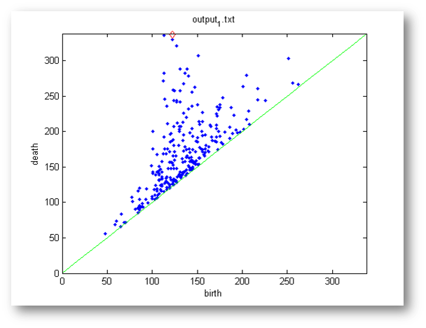
The green line is the diagonal and the typical (birth,death) type points are plotted in blue. Points with infinite persistence (meaning, those which have a death equalling -1 in the Perseus output file) are plotted as red diamonds above their birth times.
Software License and Citations
Perseus is free software: you can redistribute it and/or modify it under the terms of the GNU General Public License as published here by the Free Software Foundation. This program is distributed in the hope that it will be useful, but without any warranty; without even the implied warranty of merchantability or fitness for a particular purpose. See the GNU General Public License for more details.
If Perseus was useful in your research work, please cite it! The following paper contains the main ideas from which the Morse-theoretic simplification engine of Perseus is derived:
Konstantin Mischaikow and Vidit Nanda. Morse Theory for Filtrations and Efficient Computation of Persistent Homology. Discrete & Computational Geometry, Volume 50, Issue 2, pp 330-353, September 2013.
And if you also want to cite the software itself, please use the following:
Vidit Nanda. Perseus, the Persistent Homology Software. http://www.sas.upenn.edu/~vnanda/perseus, Accessed DD/MM/YY.
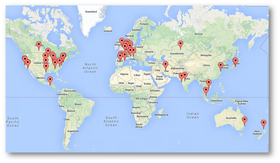
And finally, you might want to try locating yourself on this map which highlights those parts of the world where Perseus was recently downloaded: